In this article, we present a set of metrics that can be used to compare and evaluate different methods and trained models for classification problems. In our article, Machine Learning Classification in Python – Part 1: Data Profiling and Preprocessing, we introduce different classification methods whose performance can be compared with the metrics described here.
The Cases in Detail
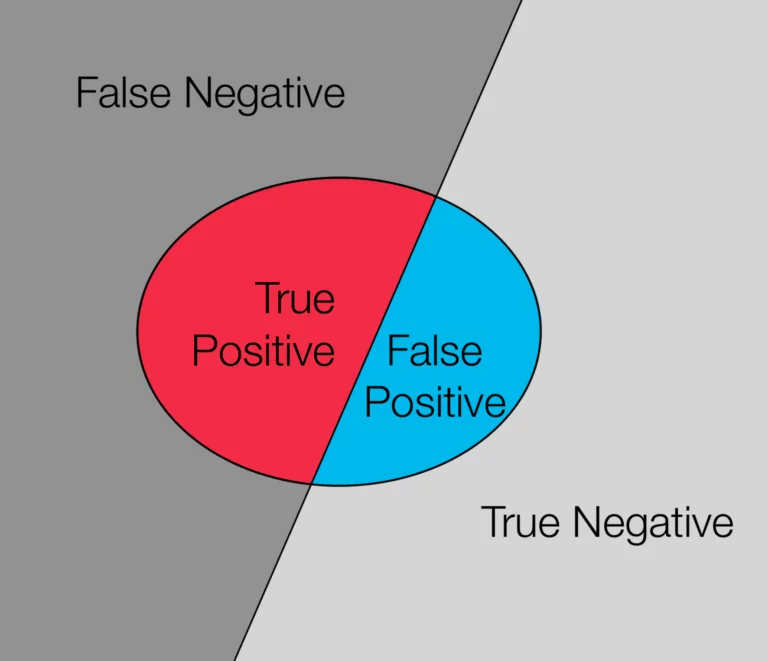
These cases all relate to the predicted target of an object to be classified. Below we list all cases together with their meaning.
- False-negative: When a data point is classified as a negative example(say class 0) but it is actually a positive example(belongs to class 1).
- False-positive: When a data point is classified as a positive example(say class 1) but it is actually a negative example(belongs to class 0).
- True-negative: When a data point is classified as a negative example(say class 0) and it is actually a negative example(belongs to class 0).
- True-positive: When a data point is classified as a positive example(say class 1) and it is actually a positive example(belongs to class 1).
Example: Transfer of Passenger Data to the BKA
To clarify the terms, we will look at an article on the transfer of passenger data to the Federal Criminal Police Office (BKA) of the SZ dated 24 April 2019. Since 29 August 2018, passenger data has been automatically transmitted to the BKA for evaluation. The data consists of the passenger’s name, address, payment data, date of travel, time of day, departure airport, and destination airport, and this information is stored in the Passenger Name Record.
This data is to be used to identify wanted offenders and suspects. In the future, this data will not only be used to identify criminals but will also be used in predictive policing. Predictive policing is the analysis of past crimes to calculate the probabilities of future crimes. The aim is to identify patterns, such as the burglary rate in a residential area, in order to be able to deploy police forces in a more targeted manner.
False Positives with Large Amounts of Data
Since the beginning of the survey until March 31st, 2019, a total of 1.2 million passenger data had been recorded and transferred. Of these, an algorithm had classified 94,098 air travelers as potentially suspicious. All hits are then checked by officials for accuracy and it turned out that only 277 of these hits were true positives. The remaining 93,821 classified suspects were false positives. The travelers from the remaining numbers, who have not been classified as suspects, can usually not be determined accurately (false negatives). The rest of the data, which was not properly classified as a match, is the true negative.
The article criticizes the high rate of false positives. This would often lead to people being unfairly targeted by authorities, in this case, 99.71% of all hits. It should be mentioned, however, that this high error rate reduces the probability of false-negative cases. This means that at the expense of many false alarms, there are significantly fewer suspicious passengers being targeted as non-suspicious.
Frequently used Performance Metrics
Based on the number of cases that have occurred, we can look at and evaluate a classifier under different metrics. In our article we have decided to use the following metrics:
Precision
A very simple metric is precision. This is the ratio of how many objects a classifier from the test data set has correctly classified as positive to those that have been falsely classified as positive. The formula is:
(True Positives) / (True Positives + False Positives)
This metric is particularly problematic in a binary classification in which a class is over-represented in the example data record; the classifier can simply assign all objects of the data record to the over-represented class but nevertheless, would achieve relatively high precision.
Using the example of passenger data, the precision is calculated as follows:
277 / (277 + 93.821) = 0,29%Recall
In contrast to Precision, the Recall Score, also known as the hit rate, indicates the proportion of all positive objects that are correctly classified as positive. This means that we get a measure to determine how many positive targets are recognized as such. The formula is:
(True Positives) / (True Positives + False Negatives)
F-Score
The F-Score combines Precision and Recall to obtain the best possible estimate of how accurately the targets of the objects are determined.
The F-Score is calculated using the harmonic mean of the formula:
F = 2 * (Precision * Recall) / (Precision + Recall)
Since we have no information about the False Negatives in our example, we are unable to determine Recall and F-Score. In our article, however, we have this information, and we can calculate both metrics.
Advanced Metrics – Receiver Operating Characteristic
The last metric we use is the Receiver Operating Characteristic curve. This indicates how reliably the classifier achieves its results. The ratio of the hit rate to the false-positive classified data as a function of a threshold value is displayed in this graph…
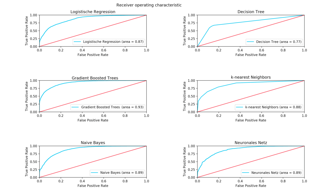
This threshold designates when an object is assigned to one or the other class. The threshold value in the lower-left corner of the graph is the largest, which means that the model only assesses the target of an object as positive if an object belongs to the target with absolute certainty. Thus, the false-positive rate approaches 0. The more one approaches the upper right corner, the lower the threshold and the more likely it is that the model falsely classifies an object as positive even though it was actually negative (False Positive). The area under curve thus serves as a metric for the quality of a tested model.
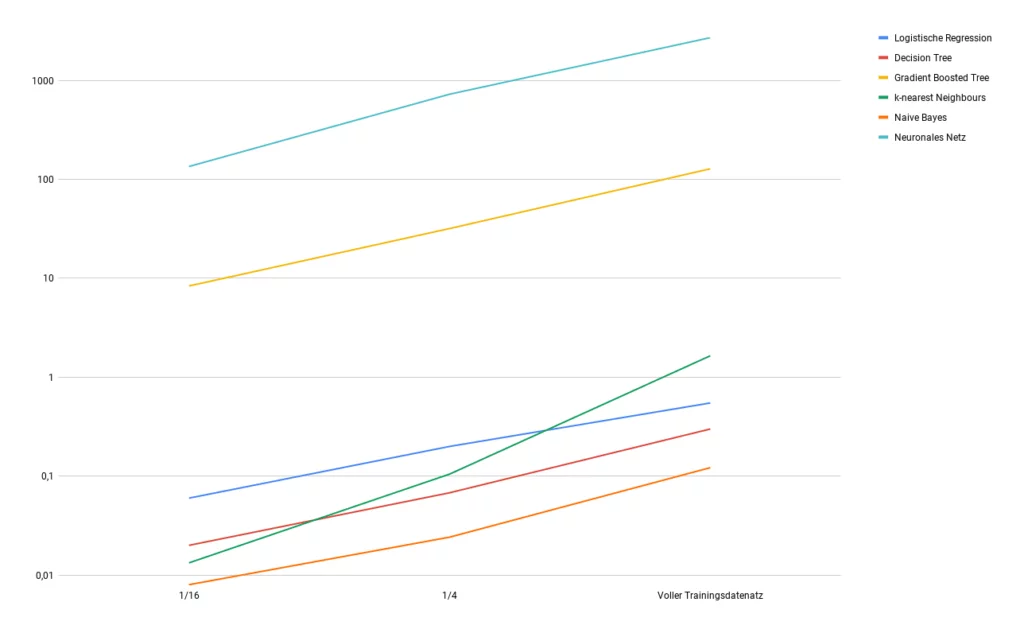
Time
Although the time required for training does not provide any indication of the quality of a classifier, it is often important to consider how quickly a classifier can be trained. The different procedures are of different complexity, which means that the differences in time and effort can be significant.
These time differences can grow exponentially with increasing data size, which is why the aspect of the time a classifier takes to reach a certain accuracy cannot be neglected, especially when working with very large amounts of data. To illustrate this aspect, we have trained our models on reduced data sets and measured the temporal differences. We obtained the following result.