
This is the second part of our series Automated Classification in Python where we use several methods to classify the UCI Machine Learning record “Adult”. In this article, after generating data from Part 1, we will discuss in more detail how we implement the different models and then compare their performance.
Classification
We use different scikit-learn models for the classification. The scikit-learn library is open-source and provides a variety of tools for data analysis. Our goal is to compare the performance of the following models: Logistic Regression, Decision Trees, Gradient Boosted Trees, k-Nearest Neighbors, Naive Bayes, and a neural net. Below we briefly summarize the methods used.
In general, the models use the training record to create a function that describes the relationship between features and targets. After training, we can apply this function to data outside the training dataset to predict its targets. More about how these feature works are summarized in our blog. Below we show our implementation of a model using the following code example:
def do_decision_tree(self):
    """ Return a decision tree classifier object. """
    clf = tree.DecisionTreeClassifier()
    return clf.fit(self.x_train, self.y_train)Code language: PHP (php)
We create a scikit-learn Decision Tree Classifier object and then train it on our training dataset.
With the scikit-learn method “predict,” it is possible to determine a model for single data or an entire data set. Based on the results obtained, we determine the performance of the model.
Classification Models
In this section, we briefly summarize the operation of each procedure. For a more detailed explanation of the model, we have linked the appropriate article from our blog and the scikit-learn documentation.
Logistic Regression
Logistic regression transforms a linear regression into a sigmoid function. Thus, logistic regression always outputs values between 0 and 1. In general, coefficients of the individual independent features are adjusted so that the separate objects can be assigned to their targets as accurately as possible.
Decision Tree
Decision tree models are simple decision trees in which each node examines an attribute, after which the next node retrieves an attribute. This happens until a “leaf” is reached that indicates the respective classification case. For more information on Decision Trees, see our article on classification.
Gradient Boosted Trees
Gradient Boosted Trees are models that consist of several individual decision trees. The goal is to design a complex representation out of many simple models. The loss function is optimized for a differentiable loss function by the coefficients of the individual trees so that the loss function is as small as possible.
k-nearest Neighbors
In the k-nearest Neighbors model, the individual objects are viewed in a vector space and classified in relation to the k closest neighbors. A detailed explanation of this model can be found in our article on classification.
Naive Bayes
The Naive Bayes model considers objects as vectors whose entries each correspond to a feature. The probability of each entry belonging to the target is determined and summed up. The object is assigned to the target whose summed probability is highest. Further information on the Naive Bayes model can also be found in our article on classification.
Neural network
Neural networks consist of one or more layers of individual neurons. When training a neural network, the weighted connections are adapted in such a way that a loss function is minimized. We have summarized more information on the structure and function of neural networks in our article, “What are artificial neural networks?”
Performance Determination
To determine the performance of our models, we wrote a function, “get_classification_report”. This function gives us the metrics; precision, recall, F-Score, and the area under the ROC curve, as well as the required key figures, which we describe in detail in our article, by calling the scikit-learn function, “metrics.classification_report” and “metrics.confusion_matrix”.
def get_classification_report(self, clf, x, y, label=""):
        """ Return a ClassificationReport object.

        Arguments:
        clf: The classifier to be reported.
        x: The feature values.
        y: The target values to validate the predictions.
        label: (optionally) sets a label."""

        roc_auc = roc_auc_score(y, clf.predict_proba(x)[:,1])
        fpr, tpr, thresholds = roc_curve(y, clf.predict_proba(x)[:,1])
        return ClassificationReport(metrics.confusion_matrix(y, clf.predict(x)),
        metrics.classification_report(y, clf.predict(x)), roc_auc, fpr, tpr, thresholds , label)Code language: PHP (php)
Only the receiver operating characteristic is obtained in the form of a graph that is generated with the help of the Python library matplotlib and the scikit-learn functions “roc_auc_score” and “roc_curve”.
Evaluation
Finally, we discuss how the models have performed on our data.
| Klassifikator | Precision | Recall | F-Score | Area under Curve | Trainingszeit (Sekunden) |
| Logistic Regression | 83% | 84% | 83% | 87% | 0,8 |
| Decision Tree | 82% | 82% | 82% | 77% | 0,5 |
| Gradient Boosted Trees | 88% | 88% | 87% | 93% | 142,9 (2 Minuten) |
| k-nearest Neighbors | 84% | 84% | 84% | 88% | 2,1 |
| Naive Bayes | 84% | 83% | 83% | 89% | 0,1 |
| Neuronal Networks | 83% | 83% | 83% | 89% | 1.746 (29 Minuten) |
A direct comparison shows that neural networks need very long training times in order to achieve adequate results. With our settings, the training lasted about 29 minutes and a precision of 83% was achieved. In contrast, the Naive Bayes classifier achieved the same accuracy in just one-tenth of a second.
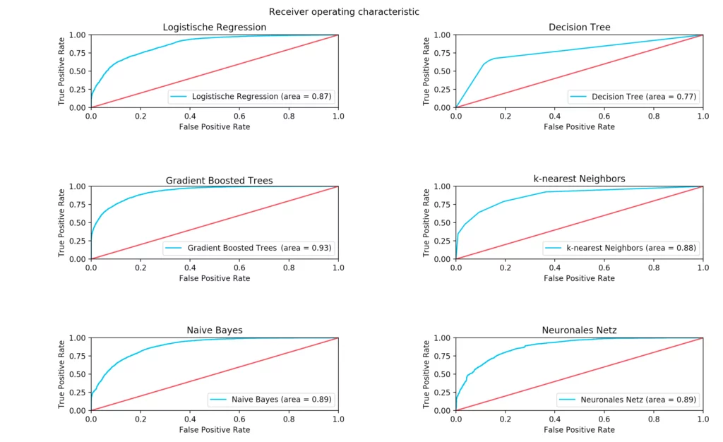
The best result was achieved with the Gradient Boosted Trees. This classifier managed to achieve a precision of 88% in 143 seconds. In addition to the relatively poor result of the neuronal net for the required training duration, it must be said that our model was most likely not chosen optimally.
In addition, the training of the neural net and the gradient boosted trees weren’t done on GPUs, which would have reduced the training duration.


