
This article, together with the code, has also been published in a Jupyter notebook.
In this article, we show different methods for clustering in Python. Clustering is the combination of different objects in groups of similar objects. For example, the segmentation of different groups of buyers in retail.
Clustering compares the individual properties of an object with the properties of other objects in a vector space. The goal of this vector space is to extrapolate relationships. The individual vectors, which represent the different properties of objects, are clustered according to their proximity to the vectors of other objects. In principle, any metric is allowed to determine the proximity of two vectors. Mostly, however, the Euclidean distance, or squared Euclidean distance (L2 norm), is used.
Often, unsupervised learning models are used for clustering. This offers an advantage from the beginning that no, or rather, only a few assumptions about the found clusters have to be made. In this article, we focus only on models that are the most common. The one disadvantage of these models is that finding a basis for assessing the result is necessary in order to be able to compare and evaluate the individual procedures.
You can find a summary of the different clustering procedures in our blog.
Validation of Clustering Results
It is difficult to objectively evaluate a clustering result, for the reason that a clustering algorithm can be discriminatory; the resulting groups can emerge by a matter of interest. If there were already a division of the objects of a data set into groups, clustering would be redundant. But as this grouping is unknown, it is difficult to say whether or not a cluster is well chosen. However, there are some methods that can be used to distinguish, at least better from worse, clustering results. By using multiple methods, finding a cluster becomes more significant. Below we have compiled a list with the most common methods.
Elbow Method
The elbow method is suitable for determining the optimal number of clusters in k-means clustering. In this case, the number of clusters is plotted in a diagram on the x-axis and the sum of the squared deviations of the individual points to the respective cluster center is plotted on the y-axis. If an elbow should be visible on the graph, this point is the optimal number of clusters. Because from this point on, the meaningfulness of the individual clusters decreases because the sum of the squared deviations only changes slightly.
Gap Statistic Method
The Gap Statistic Method compares the deviations of the individual objects within a cluster in relation to the respective center. The separation of the objects is compared with a random distribution. The further away from the points are from the random distribution, depending on the number of clusters, the better the respective number of clusters.
Calinski-Harabasz Index
The Calinski-Harabasz Index correlates with the separation and compactness of the clusters. Thus, the variance of the sums of squares of the distances of individual objects to their cluster center is divided by the sum of squares of the distance between the cluster centers and the center of the data of a cluster. A good clustering result has a high Calinski-Harabasz Index value.
Silhouette Method
The silhouette method compares the average silhouette coefficients of different cluster numbers. The silhouette coefficient indicates how well the assignment of an object to its two nearest clusters, A and B, fails. Cluster A is the cluster to which the object was assigned.
The silhouette coefficient is calculated by taking the difference of the distance of the object to the cluster B from the distance of the object to the cluster A. This difference is then weighted with the maximum distance of the object to clusters A and B. The result S (object) can be between -1 and 1. If S (object) <0, the object is closer to cluster B than to A. Therefore, clustering can be improved. If S (object) ≈ 0, then the object lies in the middle of the two clusters. Thus, clustering is not very meaningful. The closer S (object) approaches 1, the better the clustering. The silhouette method searches for the number of clusters for which the average silhouette coefficient is highest.
Clustering
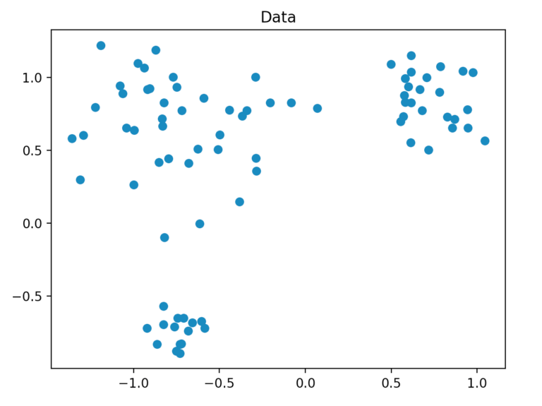
First, we will generate a dataset to cluster the data.
Data Generation
We generate our dataset so that it consists of a total of 80 two-dimensional points, which are randomly generated by three points within a defined radius. For this, we use the method “make_blobs” of scikit-learn.
Clustering Process
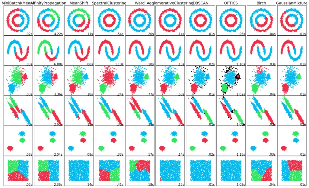
Now that we’ve generated our data, we can start the actual clustering. For this, we use the methods k-means, DBSCAN, HDBSCAN, and OPTICS. These methods all originate from the scikit-learn library, with the exception of HDBSCAN. However, for the HDBSCAN process, there is also a ready-made library that we have used. K-means is one of the partitioning methods and the remaining methods are called density-based methods. Fundamentally, HDBSCAN and OPTICS are just upgraded versions of the DBSCAN. With the method “fit_predict” of scikit-learn, we determine with each model the relationship of the points to a cluster.
At this point, we briefly introduce the methods used and explain how they work.
k-means
The k-means method divides the data into k parts. This is done by minimizing the sum of the squared deviations of the individual points from the cluster centers. On the one hand, the problem with this method is that the number of clusters has to be determined in advance, and on the other hand, this method can deal poorly with data sets of varying densities and shapes. As a result, it is often not suitable for real data records. Likewise, the method can not detect noise objects, that is, objects that are far removed from a cluster and can not be assigned to it.
DBSCAN
DBSCAN stands for “Density-Based Spatial Clustering of Applications with Noise”. The basic assumption of the DBSCAN algorithm is that the objects of a cluster are close together. There are 3 types of objects:
- Core objects are objects that are self-dense.
- Density-reachable objects are objects that are not themselves dense, but accessible from a core object.
- Noise points are objects that are not reachable from any other point.
Thereby a parameter epsilon and a parameter minPoints are defined. Epsilon determines the distance at which a point can be reached from a second point, namely, when its distance is less than epsilon. MinPoints determines when an object is dense, ie: how many objects within the distance epsilon have to be in the radius around one point.
HDBSCAN
HDBSCAN stands for “Hierarchical Density-Based Spatial Clustering” and is based on the DBSCAN algorithm. HDBSCAN extends this by transforming the DBSCAN algorithm into a hierarchical clustering algorithm. Therefore, it does not need a distance epsilon to determine the clusters. This makes it possible to find clusters of different densities and thus to remedy a major vulnerability of DBSCAN.
HDBSCAN works by first setting a number k. This determines how many neighborhood objects are considered when determining the density of a point. This is a significant difference compared to the DBSCAN algorithm. DBSCAN looks for neighbors at a given distance and HDBSCAN searches for the distance from which k objects are in the neighborhood.
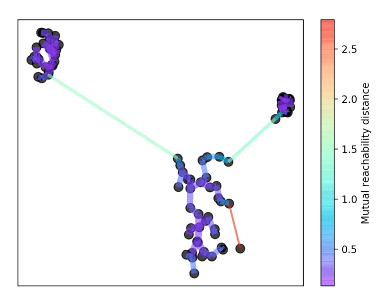
After this number k, the core distance is determined for each point. This is the smallest distance with which k objects can be reached. In addition, a reachability metric is introduced. This is defined as the largest value of either the core distance of point A, the core distance of point B, or the distance from point A to point B. This reachability metric is then used to form a minimum spanning tree. With the help of this spanning tree, the name-giving hierarchy is now formed.
For this, the longest edge is always removed from the tree. Then the hierarchy is summarized by dropping the individual points from the hierarchy depending on the distance.
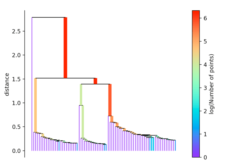
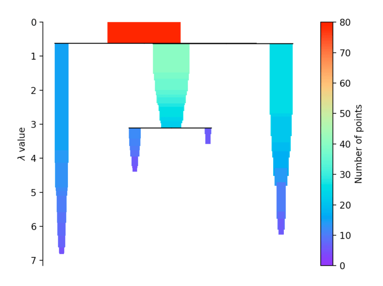
If more than initially defined min_cluster_size points fall out at a distance, they form a new subtree. Then, the method selects the clusters that have the greatest stability. The stability of a cluster is found by calculating the sum of the reciprocals of the distance from which a point falls from a cluster for all points of a cluster. In other words, if there are many points close to the cluster center, the cluster has high stability. In the picture, it is recognizable by the large area.
Evaluation
For our evaluation, we decided to use the Calinski-Harabasz index, the silhouette method, and, for the k-means clustering specifically, the elbow method.
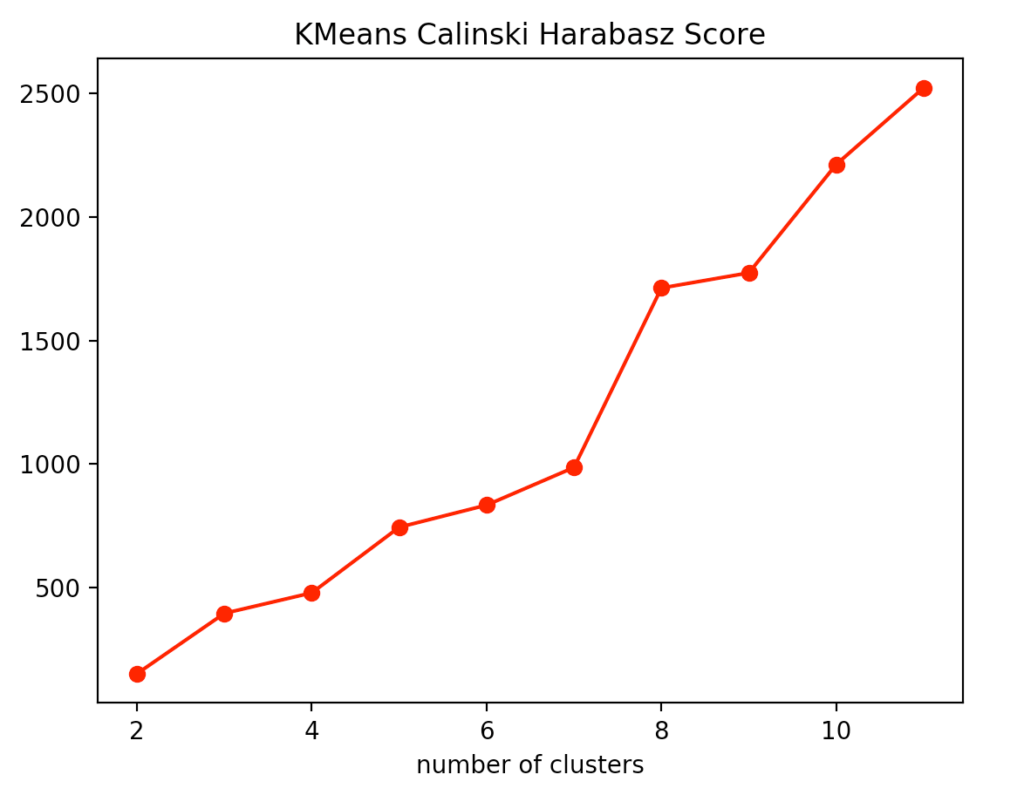
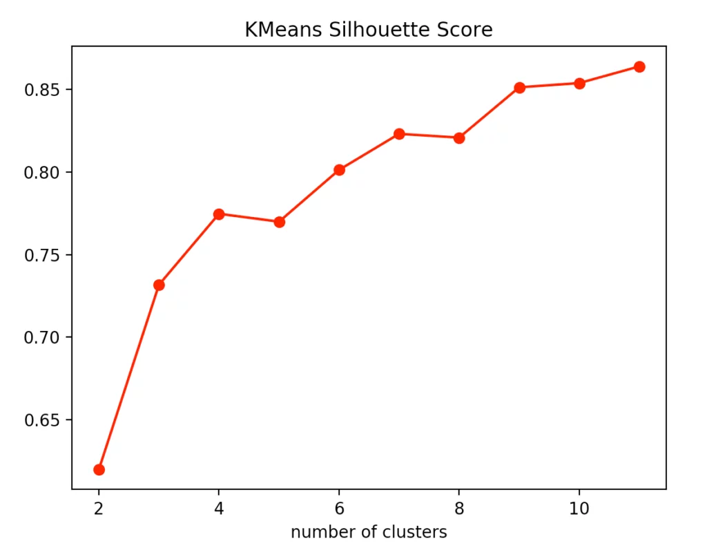
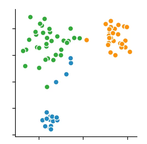
If you look at the individual metrics for k-means clustering, you find that the optimal number of cluster centers is 3. Although the silhouette method suggests that a fourth cluster would be quite useful, the Elbow method speaks against it, as a fourth cluster forms no elbow and thus provides no significant added value. Add to that the Calinski-Harabasz index, and you can see that the fourth cluster scores only slightly higher. From this, we conclude that three is the optimal number of clusters for k-means clustering on our dataset. This result also makes sense, considering that we have generated our data by 3 points.
For the other two clustering methods, we can not predetermine the number of clusters to find but merely specify the parameters by which the algorithms find the clusters. So we decided to set the distance epsilon for the DBSCAN method and only to vary the number of minPoints.
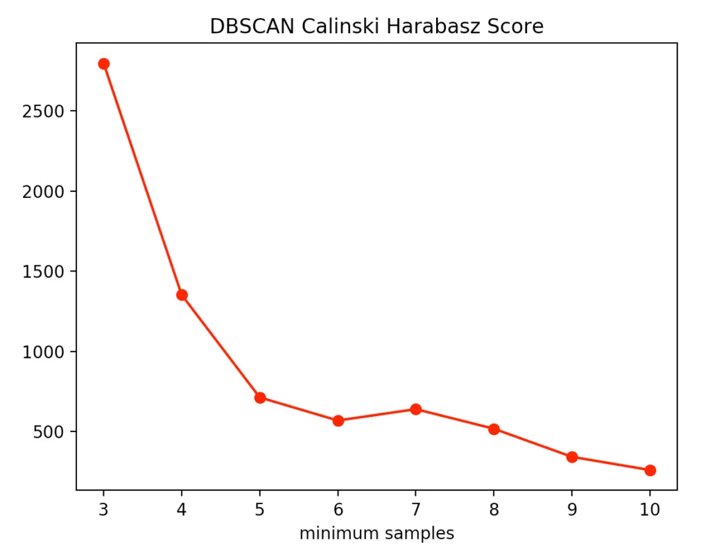
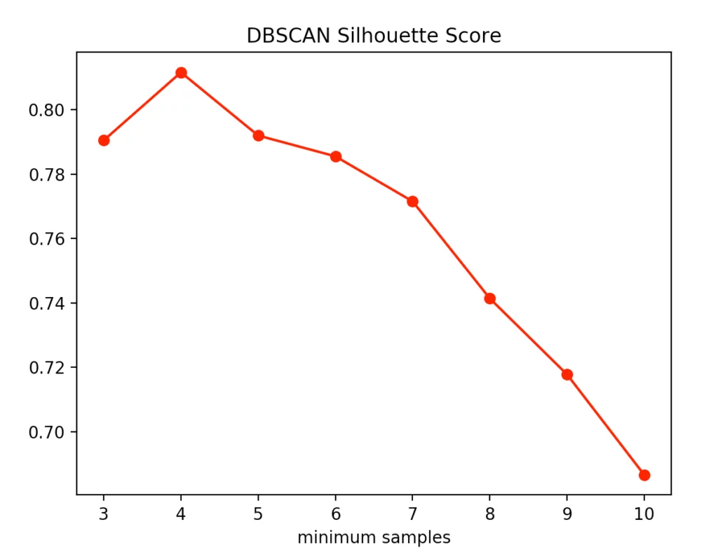
The silhouette method indicated four minPoints. On the other hand, the Calinski-Harabasz Index argues for only three minPoints. Since the difference between three and four minPoints is lower in the silhouette method than in the Calinski-Harabasz index, we decided to set the value to three. The result is the following clustering:
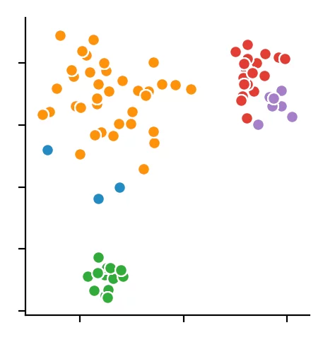
We recognize that the algorithm has chosen 4 cluster centers. It becomes clear that the DBSCAN algorithm has difficulties with different dense clusters.
With the HDBSCAN method, we vary the smallest cluster size. This is the number of points required by the hierarchical method to regard one or more separated points as new clusters. Here are the results for the Calinski-Harabasz Index and the Silhouettes method.
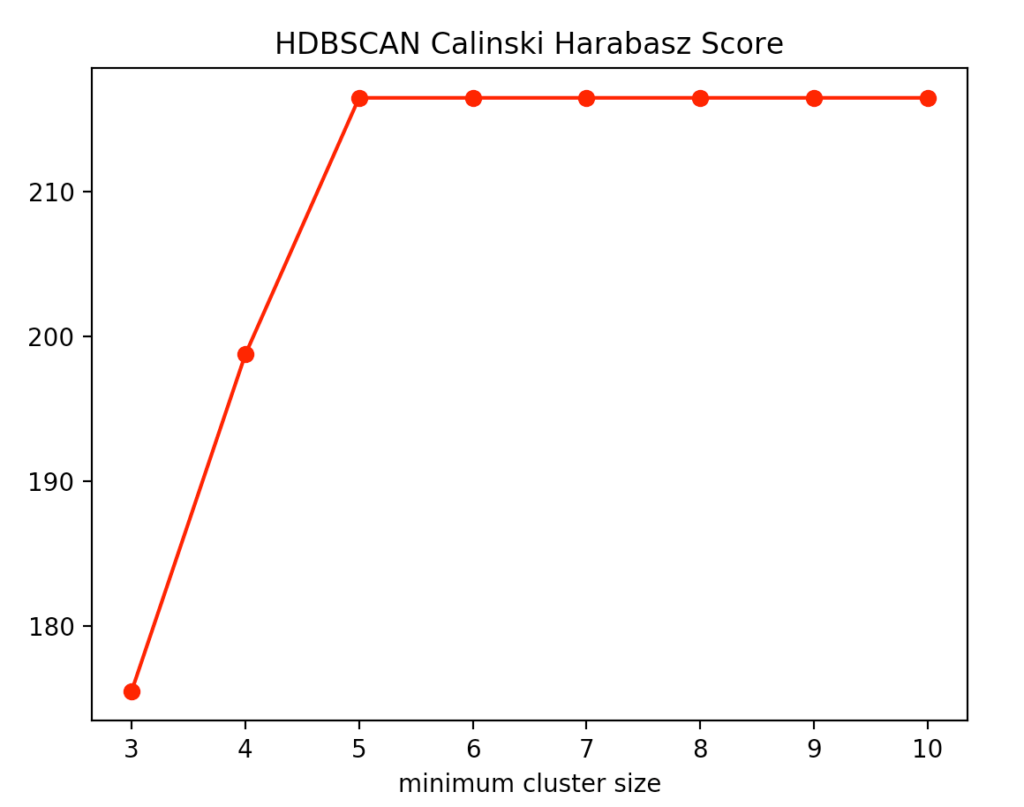
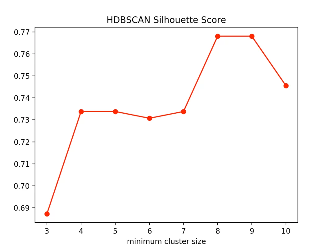
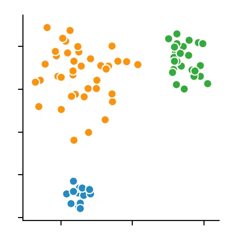
We recognize that the optimal size is between four and five points. We decided to use four and get the following result.
Conclusion
It should be clear that clustering results on a dataset can be difficult to classify. There are many other methods that have also produced different solutions. The metrics for the validation of the clustering results are only partially suitable. It is always useful to use a variety of metrics to help compare them with each other in order to find the most suitable algorithm for a particular application. It also helps to fine-tune the parameters in the interest of obtaining the best result. Despite the weaknesses mentioned above, clustering methods make it possible to divide higher-dimensional data into groups.


