Clustering with Machine Learning — A Comprehensive Guide

The term clustering (in machine learning) refers to the grouping of data: The eponymous clusters. In contrast to data classification, these are not determined by certain common features but result from the spatial similarity of the observed objects (data points/observations). Similarity refers to the spatial distance between the objects, represented as vectors. There are various methods to determine this distance, such as the Euclidean or the Minkowski metric.

However, this fact already indicates that there is no uniform and clearly defined methodology for cluster determination. In this article we therefore

1. will introduce you to the various methods and algorithms for cluster analysis as well as their advantages and disadvantages.
2. In addition, we will look at the applications for clustering (including their problem areas)
3. plus a concrete example of a cluster analysis.

This will allow you to form your own opinion about which of these algorithms is best suited for your own cluster analysis (in machine learning). But enough of the long preliminary remarks – now have fun reading through and becoming more informed.

Table of contents:

1. What is cluster analysis (clustering)?
2. What is a cluster?
3. Which methods (and algorithms) are available for cluster analysis?
   • Hierarchical clustering
   • Partitioning clustering (centroid-based)
   • Density-based clustering
   • Distribution-based clustering
4. Validation of clustering results
5. Applications of cluster analysis for Machine Learning
6. Example of a cluster analysis
7. Obstacles of clustering in Machine Learning

1. What is cluster analysis (clustering)?

Cluster analysis (clustering) is a non-supervised method of machine learning. It involves the automatic identification of natural data groups (the clusters). An unsupervised learning method is one in which we draw conclusions from data sets consisting of input data without labeled answers – using labeled data sets, on the other hand, would be the method of data classification already mentioned.

Thus, in contrast to supervised learning (such as predictive modeling), clustering algorithms simply interpret the input data. Based on this analysis, they then subsequently determine the natural groups already mentioned for the selected characteristics. For this purpose, the data points used (observations) are evaluated individually in order to assign each of them to a specific group.

• Consequently, data points that are in the same group should have similar properties and / or characteristics.
• Data points in different groups, on the other hand, should have very different characteristics.  

Clustering techniques are used when no classification should be predefined, but the data should be divided into natural groups. They often represent the first step on the way to understanding data sets.

Clustering can be used in data analysis for gaining knowledge and understanding pattern recognition, in order to learn more about the data domain under investigation.  Clustering can also be useful as a form of feature engineering, where existing and new data points can be mapped together and associated with an already identified cluster. Other possible applications of cluster analysis in machine learning include:

• market segmentation,
• social network analysis,
• grouping of search results,
• medical image processing,
• image segmentation,
• or anomaly detection.

The evaluation of identified clusters is often subjective and may require an experienced expert, although in principle a wide variety of quantitative metrics and techniques exist. Typically, such clustering algorithms are therefore first tested experimentally on theoretical data sets with predefined clusters to determine their practicality.

2. What is a Cluster? 

The definition for the term “cluster” cannot be precisely defined. This is one of the reasons why there are so many clustering algorithms. However, there is a common denominator: A group of data points with similar properties and/or characteristics. Furthermore, the following requirements should be met:

1. Data points that are in the same cluster must be as similar as possible.
2. Data points that are in different clusters must be as different as possible.
3. The metrics for similarity and dissimilarity must be clearly defined and have a concrete relation to practice.

However, different approaches (as already mentioned) use different cluster models – and for each of these, in turn, different algorithms can be specified. The definition of a cluster, as found by different algorithms, varies considerably in its properties. We have listed the most important algorithms/methods for cluster analysis (including the resulting cluster types) in the following chapters.

3. Which methods (and algorithms) are available for cluster analysis? 

There are various approaches to cluster analysis, each of which has its own advantages and disadvantages. They also lead to different results – i.e. classes of clusters. However, they all use distance (dissimilarity) and similarity as the basis for clustering. In the case of quantitative characteristics, distance is preferred in order to identify the relationship between the individual data points. Similarly, on the other hand, clustering is preferred when it comes to qualitative characteristics.

In addition, each cluster analysis method follows the following basic steps:

1. Feature extraction and selection: Extraction and selection of the most representative features from the original data set.
2. Design of the clustering algorithm: According to the characteristics of the problem being addressed by the data analysis.
3. Result evaluation: Evaluation of the clusters obtained and assessment of the validity of the algorithm.
4. Result interpretation: What is the practical explanation for the clustering result?

In most cases, in order to achieve the best results for a data set, one has to try out several of these methods with different parameters and then decide on one. There is no single method that works best in general. The most common unsupervised learning methods include:

3a) Hierarchical Clustering

The basic idea of this type of clustering algorithm is to reconstruct the hierarchical relationship between the data in order to group them based on it. In the beginning, either the set of all data points in total (top-down / a single large cluster) or the set of all individual data points (bottom-up / a single cluster for each data point) is assumed to be the cluster.

1. In the top-down method, the central cluster is subsequently divided by selecting the data point furthest away from its center as the second cluster center. The algorithm then assigns all the other data points to the closer center, forming two separate clusters. This process can then be continued even further to increase the number of clusters.
2. In the bottom-up method, the closest clusters are combined into a new cluster in order to reduce their number step by step.

With both methods, it is difficult to define the way in which the distance between the individual data points is determined. On the other hand, how far do you want to divide or combine the clusters. Finally, one should not repeat the process until as many clusters as individual data points or only one cluster remains – and thus end up at the beginning of the respective another approach (top-down / bottom-up).

Hierarchical clustering creates a tree structure and is, therefore (unsurprisingly) well suited for hierarchical data, such as taxonomies. Typical algorithms here are, for example, BIRCH, CURE, ROCK, or Chameleon.

Advantages and disadvantages of hierarchical clustering methods for Machine Learning:

Advantages:

• Suitable for data sets with arbitrary characteristics.
• The hierarchical relationship between the clusters can be easily identified.
• Scalability is generally relatively high.

Disadvantages:

• Relatively high time complexity in general.
• The number of clusters must be preselected.

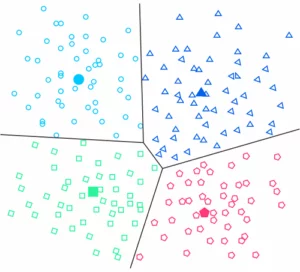
3b) Partitioning clustering (centroid-based)

In partitioning clustering, first, a number k is defined which specifies the number of clusters. Based on this number, the algorithm determines k cluster centers. Subsequently, the centers obtained are shifted in such a way that the metric of the data points to their nearest cluster center is minimized. Thus, in contrast to hierarchical clustering, centroid-based clustering organizes the data in non-hierarchical clusters.

The basic idea of this type of clustering algorithm is to consider the mean between all the data points as the center of the respective cluster. K-means and K-medoids are the two best-known of such algorithms. The core idea of K-means, for example, is to continuously update the center of the cluster through iterative calculation. This iterative process continues until certain convergence criteria are met. Other typical clustering algorithms based on partitioning are PAM, CLARA, or CLARANS.

Advantages and disadvantages of partitioning clustering methods for Machine Learning:

Advantages:

• Relatively low time complexity and generally high computing efficiency.
• The association of the individual data points to a cluster can be changed during clustering.

Disadvantages:

• Not suitable for non-convex data.
• Relatively sensitive to outliers.
• Easily drawn into a local optimum.
• The number of clusters must be predefined. Therefore, to achieve optimal results, one has to run the algorithm with different values and then select one of them.
• The clustering result depends on the number of clusters.

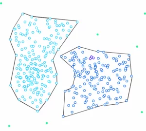
3c) Density-based clustering

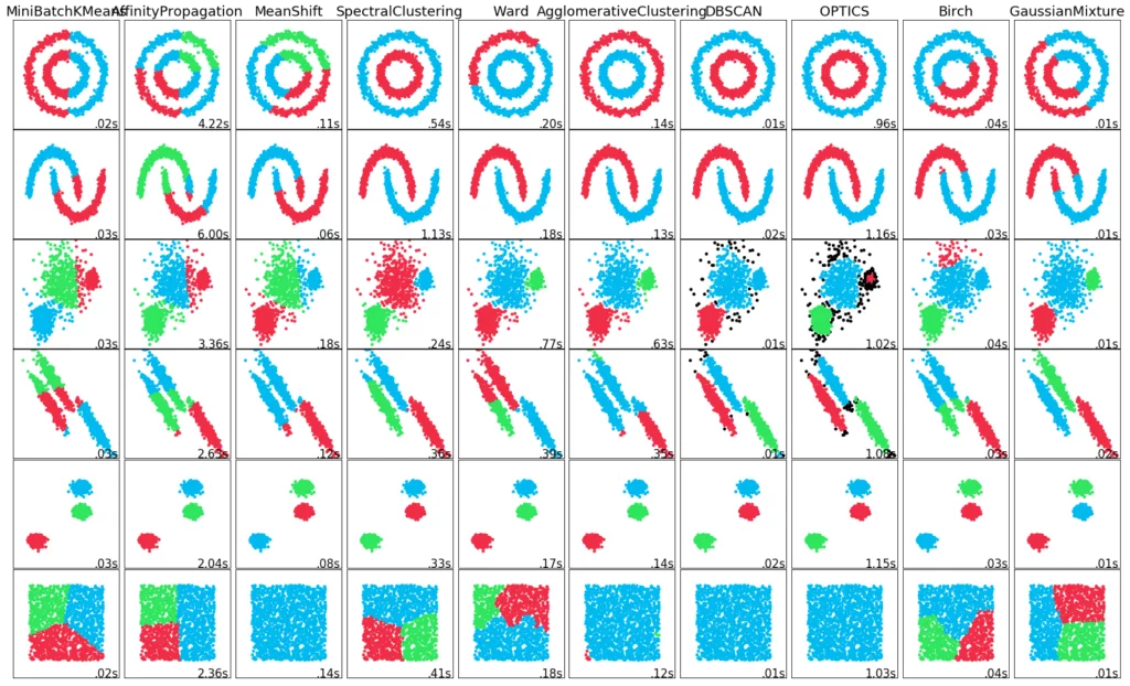
The basic idea of these types of clustering algorithms is that data points located in a region of high data density are considered to belong to the same cluster. Typical of these algorithms are DBSCAN, HDBSCAN, OPTICS, and Mean-Shift. We will briefly explain the first two in more detail here, as we will use them later in our clustering example.

The most popular of the previously mentioned methods is DBSCAN. In this method, a distance ε is determined together with a number k. Data points that have k neighboring objects with a distance smaller than epsilon (ε) represent core objects that are combined to form a cluster center. Data points that are not core objects but are located near a center are added to the cluster. Data points that do not belong to any cluster are considered noise objects.

HDBSCAN stands for “Hierarchical Density-Based Spatial Clustering” – and as already mentioned, it is based on the DBSCAN algorithm. However, it extends it by transforming it into a hierarchical clustering algorithm. Therefore, it does not need a distance ε to determine the clusters. This makes it possible to find clusters of different densities, thus eliminating a major weakness of DBSCAN.

In the HDBSCAN method, first, a number k is determined. This number is used to determine how many neighborhood objects are considered when determining the density of a given spot. This is already a decisive difference compared to DBSCAN. DBSCAN searches for neighbors at the given distance ε, whereas HDBSCAN searches for the distance from which k objects lie in the neighborhood.

According to this number k, the core distance is determined for each spot. This is the smallest distance at which k objects can be reached. A reachability metric is also introduced. This is defined as the largest value of either the core distance of point A, the core distance of point B, or the distance from point A to point B. This reachability metric is then used to build a minimum spanning tree.

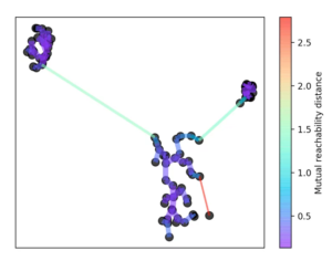
To do this, we always remove the longest edge from the tree. The hierarchy is then created by eliminating the individual points from it depending on their distance.

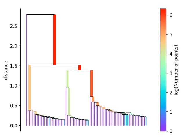
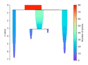
If more than the “min_cluster_size” points defined at the beginning fall out at a distance, these form a new subtree. The procedure then selects the clusters that have the greatest stability. This is determined by calculating the sum of the reciprocal values of the distance at which a point falls out of a cluster for all points of a cluster. This means that if many points are close to the center, the cluster has high stability. In the picture, this is recognizable by a large area.

Advantages and disadvantages of density-based clustering methods for Machine Learning:

Advantages:

• Clustering with high efficiency.
• Suitable for any data formats.

Disadvantages:

• Leads to a clustering result with low quality if the density of the data space is not uniform.
• Requires a very large memory space if the data volume is large.
• The clustering result is very sensitive to the predefined parameters.

3d) Distribution-based Clustering

This clustering approach assumes that the data consists of distributions (such as the Gaussian distribution). As the distance from the center of a distribution increases, the probability that a data point belongs to it decreases. The prerequisite for a distribution-based cluster analysis is always that several distributions are present in the data set. Typical algorithms here are DBCLASD and GMM.

The core idea of GMM is that the data set consists of several Gaussian distributions generated from the original data. And that the data that belong to the same independent Gaussian distribution are considered to belong to the same cluster.

Advantages and disadvantages of distribution-based clustering methods for Machine Learning:

Advantages:

• More realistic values for the probability of adherence.
• Relatively high scalability due to the change in the applied distribution and thus number of clusters.
• Statistically well provable.

Disadvantages:

• Basic assumption is not one hundred percent correct.
• Numerous parameters that have a strong influence on the clustering result.
• Relatively high time complexity.

That was the overview of the most important clustering methods in Machine Learning. However, it can be difficult to evaluate a clustering result objectively, since the algorithm is supposed to find clusters automatically. If there were already a classification of the data points into groups, clustering would be unnecessary. However, since this grouping is not known, the result determined by the algorithm must then be critically evaluated. For this purpose, various methods are available that can be used to distinguish better from worse results. In the following chapter, we will introduce you to the most common of these in more detail.

4. Validation of clustering results

To evaluate the results of a cluster analysis – especially with regard to the number of clusters obtained – there exist several methods. Some of the most common of these are explained in detail below.

4a) Elbow criterion

The Elbow criterion is very suitable for determining the optimal number of clusters in a K-means clustering. The number of clusters is plotted on the x-axis and the sum of the squared deviations of the individual points from the respective cluster center is plotted on the y-axis. If a bend (the elbow) is visible on the resulting diagram, this point is the optimal number of clusters. From this point on, the significance of the individual clusters decreases, as the sum of the squared deviations only changes slightly.

Using the “elbow” or “knee of a curve” as a cut-off point is a common approach in mathematical optimization to choose a point at which diminishing returns are no longer worth the additional costs. In clustering, this means that one should choose a number of clusters where adding more clusters no longer gives significantly better modeling of the data.

Theoretically, increasing the number of clusters improves the fitting because more of the variation is explained. However, the more parameters (more clusters) at a certain point constitutes overfitting, which is reflected by the bend in the graph. For data that actually consists of k defined groups – e.g. k points sampled with noise – clustering with more than k clusters will “explain” more of the variation (as it can use smaller, tighter clusters). However, the overfitting is that the defined groups are subdivided into further sub-clusters.

This is based on the fact that the first clusters add a lot of information (explain a lot of variation) because the data actually consists of that many groups – consequently, these clusters are necessary. However, as soon as the number of clusters exceeds the actual number of groups in the data set used, the information content decreases sharply.

The result: A sharp bend in the graph because it rises rapidly up to point k (underfitting area) and thereafter only slowly (overfitting area). The optimal range (optimal number of clusters) is therefore the point k, as already explained at the beginning.

4b) Gap Statistic

The gap statistic is also a way of approximating the optimal number of clusters (k) for unsupervised clustering. It relies on evaluating an error metric (the sum of squares within clusters) with respect to our choice of k. We tend to see that the error decreases steadily as the number of clusters increases.

However, we reach a point where the error stops decreasing (the elbow in the graph). This is the point at which we want to set our value of k as the “proper” number of clusters. While we could purely look at the diagram and estimate the elbow – better suited to do this is a formalized method: the Gap Method.

We now have this graph comparing the error rate (e.g. K-Means WCSS) with the value of k. We can only get a sense of how good each error or k-value pair is if we are able to compare the expected error for k under a zero reference distribution. In other words, if there were absolutely no signals in data with a similar overall distribution and we grouped them with k clusters, what would be the expected error?

We now want to use the gap statistic to find the value of k for which the gap between the expected error under a zero distribution and our clustering is the largest. If the data has real, meaningful clusters, we would expect this error rate to decrease faster than the calculated rate.

4c) Calinski-Harabasz-Index

The Calinski-Harabasz index (also known as the variance ratio criterion) is relatively quick to calculate – and is the ratio of the variance of the sums of squares of the distances of individual objects to their cluster center divided by the sum of squares of the distance between the cluster centers and the center of the data of a cluster. A good clustering result has a high Calinski-Harabasz score. This is because the score is higher if the clusters are dense and well separated, as it corresponds to the standard concept of a cluster.

4d) Silhouette Coefficient

The silhouette method compares the average silhouette coefficient of different numbers of clusters. The silhouette coefficient indicates how good the orientation of a data point is to its two closest clusters A and B. Thereby, cluster A is the one to which the object was assigned.

The silhouette coefficient is calculated by taking the difference between the distance of the data point to cluster B and the distance of the data point to cluster A. This difference is then multiplied with the maximum distance of the data point to cluster A and B. The result S can be between -1 and 1.

1. If S < 0, the object is closer to cluster B than to A. Accordingly, the clustering can be improved.
2. If S ≈ 0, the object is in the middle of both. Thus, the clustering is not very meaningful.
3. The closer S is getting to 1, the better the clustering. Consequently, the silhouette method looks for the number of clusters for which the average silhouette coefficient is highest.

5. Applications of cluster analysis for Machine Learning

Since clustering methods are able to make abstract connections in data visible, which the human brain does not perceive so clearly, they are nowadays used in many areas of Machine Learning. The areas of application include, for example:

1. Market research: Clustering is widely used in this field, e.g. to analyse data from surveys. Here, customers are divided into groups to which optimal product or advertising placements are subsequently tailored.
2. Natural Language Processing (NLP): Here, clustering algorithms enable the automated evaluation of texts and language.
3. Crime analysis: In this case, clustering allows for an efficient deployment of police and security forces, as crime hot spots can be better recognised and evaluated.
4. Identifying cancer cells: The clustering algorithms divide cancerous and non-cancerous data sets into different groups.
5. Search engines: Search engines also work with the clustering technique. The search result is created based on the object that is closest to the search query. This is done by grouping similar objects into a group that is distant from dissimilar objects. The accuracy of the result of a search query thus depends heavily on the quality of the clustering algorithm used.
6. Life sciences: In biology, cluster analysis is used, for example, to classify different species of plants and animals using image recognition technology.
7. Landscaping: The clustering technique is used to identify areas with similar land use in the GIS database. This can be very useful, for example, to determine for which purpose a certain land area should be used – i.e. for which it is most suitable.

Now that we have learned about the most important applications of cluster analysis in Machine Learning, let’s look at a practical example of such an analysis in detail.

6. Practical example for a cluster analysis

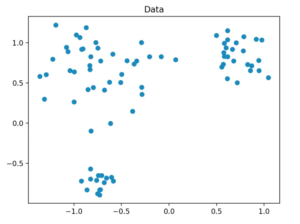
In order to carry out an exemplary cluster analysis, we must first generate a data set in order to subsequently classify its data into clusters.

6a) Data set generation

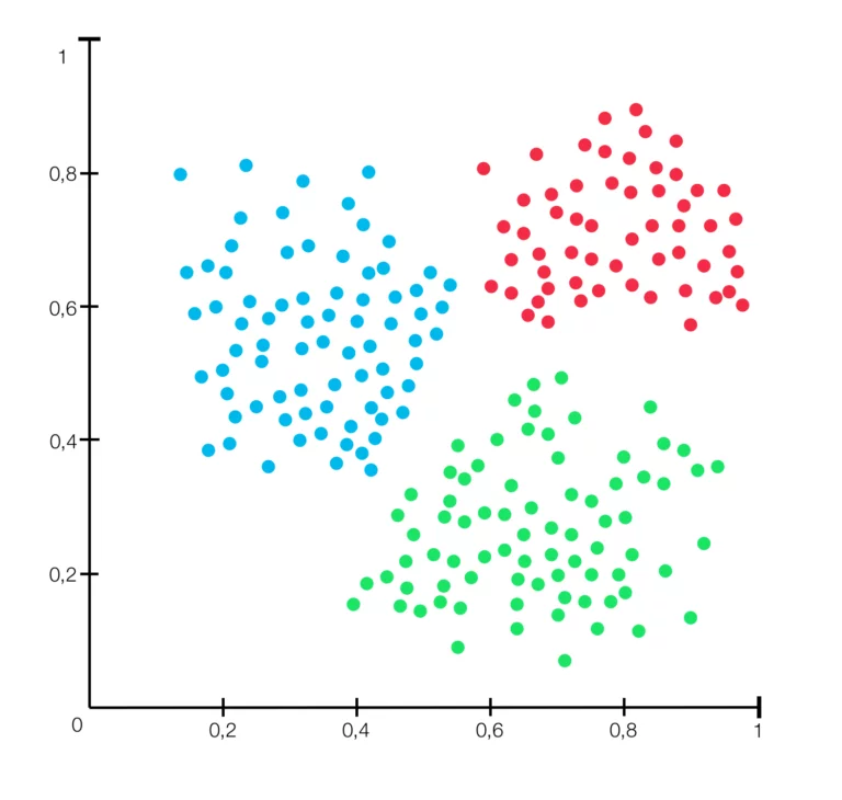
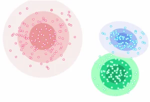
We generate our data set in such a way that it consists of a total of 80 two-dimensional data points that are randomly generated around three central points in a fixed radius. For this, we use the method “make_blobs” from scikit-learn.

6b) The clustering methods being used

After we have generated our data, we can start with the actual clustering. For this, we use the algorithms k-means, DBSCAN, and HDBSCAN. K-means is a partitioning method, while the others are density-based. HDBSCAN is based on DBSCAN. We have already presented the individual algorithms used in this example in detail in chapter 3.

With the exception of HDBSCAN, the algorithms derive from the scikit-learn library. For the HDBSCAN method, however, there is also a ready-made library available that we can use. With the “fit_predict” method from scikit-learn, we subsequently determine the assignment of the individual data points to a cluster with each model.

6c) Interpretation of our cluster analysis example

For these, we use the Calinski-Harabasz-Index and the Silhouette-Method – and for the k-means clustering in particular the Elbow-Criterion.

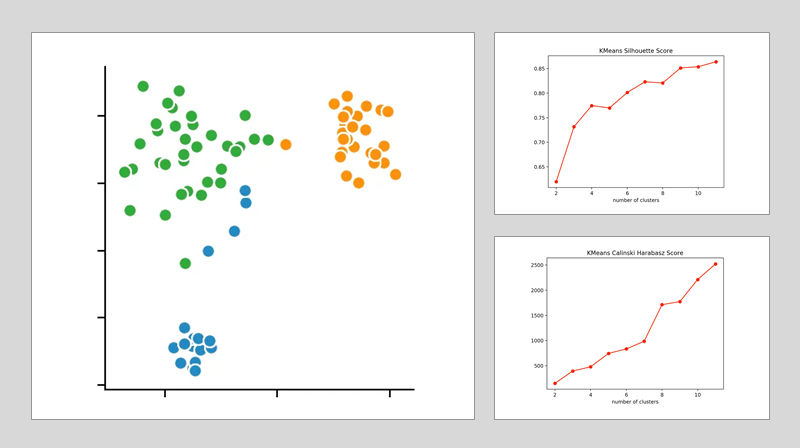
k-means-Clustering:

If we look at the individual metrics for this, we find that the optimal number of cluster centers is 3. Although the Silhouette-Method suggests that a fourth cluster would make sense, the Elbow-Criterion does not support this. In this case, a fourth cluster does not form a bend and thus offers only very limited added value.

If we now also include the Calinski-Harabasz-Index, we furthermore see that the fourth cluster only achieves a slightly higher score. From this observation, we conclude that three is the optimal number of clusters for a k-means clustering on our data set. This result also makes perfect sense when we consider that we have generated our data around 3 central points.

DBSCAN:

For the other two clustering methods, we cannot determine the number of clusters to be found in advance, but only the parameters according to which the algorithms select their number. For the DBSCAN method, for this purpose, we specify the distance ε and only vary the number of minPoints.

The silhouette method indicates the number of four minPoints. In contrast, the Calinski-Harabasz-Index suggests that only three of these should be defined. Since the difference from three to four is smaller in the Silhouette-Method than in the Calinski-Harabasz-Index, we decided to set the value at three. This results in the following clustering:

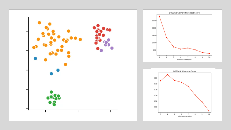
We see that the algorithm has chosen 4 cluster centers. This clearly shows that the DBSCAN method has difficulties with clusters of different densities.

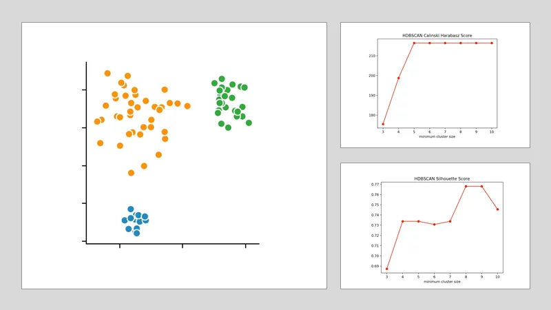
HDBSCAN:

With the HDBSCAN algorithm, we vary the smallest cluster size. This is the number of points needed in a hierarchical procedure for one (or more) isolated data points to be considered a new cluster. By applying the Calinski-Harabasz-Index and the Silhouette-Method, we discover that the optimal size is between four and five points. We decide on four and get the following clustering result.

With this example, it should have become clear that it can be difficult to check clustering results from a data set for their accuracy. There are many other methods that would also have produced different results. The metrics for validating the clustering results are only suitable to a limited extent. Therefore, it always makes sense to consult several of them and compare them with each other. This is the only way to find the most suitable algorithm for the respective application – and to optimally adjust all other parameters to it.

7. Obstacles of clustering in Machine Learning

Data mining attempts to discover patterns in large data sets. The goal of cluster analysis is thus to determine the natural groups within a large amount of collected data (data points). The use of clustering methods for machine learning has two major weaknesses:

1. With very large data sets, the key concept of clustering – the distance between individual measurements / observations – is made useless by the so-called curse of dimensionality. This makes it very time consuming for large datasets – especially if the space has multiple dimensions.
2. Shortcomings of existing (and applied) algorithms. These include:
   1. the inability to recognise whether the data set is homogeneous or contains clusters.
   2. the inability to rank variables according to their contribution to the heterogeneity of the dataset.
   3. the inability to recognise specific patterns: Cluster centers, core regions, boundaries of clusters, zones of mixing, noise or even outliers.
   4. the inability to estimate the correct number of clusters.
   5. Moreover, each algorithm is designed to find the same type of clusters. As a result, it fails as soon as there is a mixture of clusters with different properties.

Furthermore, the effectiveness of the clustering is determined by the chosen method of distance measurement. Usually, there is no universally correct result. This is due to the fact that it varies drastically depending on the different methods, each with different parameters. As explained in detail in chapter 4, it is therefore sometimes not so easy to interpret the result and to check its correctness.

Possibilities to carry out this verification would be to compare the result of the clustering with known classifications or the evaluation by a human expert. However, both options are only suitable to a limited extent, since on the one hand clustering would not be necessary if there were already known classifications. And on the other hand, human evaluations are always very subjective.

Despite their weaknesses, however, clustering methods make it possible to divide even higher-dimensional data into homogeneous groups. This makes them very suitable for data evaluation and processing in machine learning. It is only important to always consider the points just mentioned and to critically question the results (clusters) obtained.

And with that, we have already reached the end of our brief overview of the biggest obstacles of clustering for Machine Learning. This also brings us to the end of our article. We hope that the information and practical examples listed here will be helpful to you for your own software development project.

In case you need any further support, we invite you to contact us and use our experienced team for your software development – we are looking forward to your message. This way you save valuable time for your launch, which you can invest in building your own team. So that you can handle the next product development completely in-house!